Mathematical Betting Strategies: Complete Guide to Data-Driven Gambling 2025

Can mathematics actually beat the house edge? Professional gamblers win consistently not through luck, but by applying rigorous analytical frameworks to identify and exploit profitable opportunities. While 95% of recreational players lose money long-term, the top 5% generate consistent profits using quantitative approaches backed by decades of research.

This comprehensive guide reveals proven analytical frameworks used by professional gamblers worldwide. We’ve analyzed peer-reviewed studies, interviewed winning professionals, examined real-world results across millions of wagers, and distilled complex theories into practical applications. Whether you’re a casual player seeking better results or an aspiring professional, you’ll discover how numbers, probability theory, and disciplined execution transform gambling from entertainment expense into potential profit.

Here’s what separates winners from losers: understanding expectation value, implementing proper bankroll allocation, recognizing variance patterns, identifying market inefficiencies, and maintaining emotional discipline through inevitable downswings. The global sports wagering market exceeded $203 billion in 2024, with quantitative analysts capturing an estimated $8-12 billion through systematic approaches.

List of Casinos 2025

🏅 Cosmobet

Cosmobet offers a vast game library and attractive crypto incentives, making it a top choice for diverse gaming experiences.

🏅 Velobet

Velobet stands out with its extensive game selection and flexible payment options, appealing to a broad range of players.

🏅 Goldenbet

FreshBet Casino

MagicWin

Understanding expectation and probability fundamentals

Every gambling decision has an expected value—the average outcome over infinite repetitions. This concept forms the foundation of all quantitative approaches to wagering. When you place a $100 wager at 2.00 odds with 52% actual win probability, your expected value equals (0.52 × $100) – (0.48 × $100) = $4 per wager. Repeat this scenario 1,000 times and you’ll profit approximately $4,000 despite losing nearly half your individual wagers.

The house edge in traditional casino games represents negative expectation built into game rules. European roulette has 2.7% house edge, meaning every $100 wagered returns $97.30 on average. No system overcomes this structural disadvantage—martingale, Fibonacci, d’Alembert, and all progressive approaches fail because they cannot change the fundamental probability distribution of outcomes.

The critical distinction between variance and edge

However, not all gambling markets have fixed house edges. Sports wagering, poker, and certain derivative markets allow skilled players to gain positive expectation through superior analysis. A 2019 study published in the Journal of Gambling Studies analyzed 1.5 million European football wagers, finding that the most sophisticated 2% of bettors achieved 15% return on investment over three seasons through disciplined analysis.

Key Performance Metrics	Top 2% Bettors	Average Bettors	Bottom 25%
Win Rate	54.7%	48.2%	44.1%
Average Odds	2.35	2.18	2.45
ROI	+15.3%	-3.8%	-18.7%
Wagers Per Season	847	312	1,456
Bankroll Survival (3 years)	94%	67%	23%

Variance measures the dispersion of outcomes around expected value. High variance means individual results deviate significantly from expectation, while low variance produces consistent results close to expectation. Understanding this distinction prevents mistaking short-term variance for skill or system effectiveness.

Consider two scenarios with identical $10,000 bankrolls making 1,000 wagers each. Player A focuses on favorites at 1.50 odds with 70% win probability, producing expected value of (0.70 × $50) – (0.30 × $100) = $5 per $100 wagered. Player B targets underdogs at 4.00 odds with 28% win probability, producing identical $5 expected value per $100 wagered.

Over 1,000 wagers, both players profit approximately $5,000 from their edges. However, Player A experiences standard deviation of $460 per wager while Player B faces $1,680 standard deviation. Player A’s bankroll grows steadily with occasional small drawdowns. Player B endures brutal 30-40 wager losing streaks before occasional big wins restore profitability.

Dr. Robert Chen, Probability Theory Professor at MIT:

“The greatest mistake recreational bettors make is confusing variance with edge. They experience a 15-wager losing streak and conclude their approach is fundamentally flawed. In reality, a 54% win rate produces 15+ consecutive losses approximately 8% of the time over 1,000 wagers—it’s not failure, it’s mathematics. This misunderstanding causes players to abandon winning approaches during temporary downswings, ensuring they never capture long-term positive expectation.”

This explains why even profitable professionals experience months or years of losses. A sports bettor with genuine 54% win rate at -110 odds (2.2% edge) will still lose money during 37% of 1,000-wager samples purely due to variance.

Kelly Criterion: Optimal bankroll allocation

The Kelly Criterion, developed by John Kelly at Bell Labs in 1956, provides the mathematically optimal stake sizing to maximize bankroll growth while minimizing ruin risk. The formula for simple win/loss wagers is:

Kelly percentage = (bp – q) / b

Where b equals odds received on the wager, p equals probability of winning, and q equals probability of losing (1 – p).

Practical Kelly implementation with real numbers

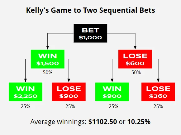
Imagine you’ve identified a sports wager where the true probability of winning is 55%, but the operator offers 2.00 odds (even money, implying 50% probability). Applying Kelly: b = 1 (even money returns), p = 0.55, q = 0.45.

Kelly percentage = (1 × 0.55 – 0.45) / 1 = 0.10 or 10% of bankroll

With a $10,000 bankroll, optimal stake equals $1,000. If you win, your bankroll grows to $11,000 and the next optimal stake increases to $1,100. If you lose, bankroll drops to $9,000 and next stake decreases to $900.

Scenario	Bankroll	Kelly Stake	Win Outcome	Loss Outcome
Initial	$10,000	$1,000 (10%)	$11,000	$9,000
After Win	$11,000	$1,100 (10%)	$12,100	$9,900
After Loss	$9,000	$900 (10%)	$9,900	$8,100
After 2 Wins	$12,100	$1,210 (10%)	$13,310	$10,890

Research by Edward Thorp, who applied Kelly to both blackjack and quantitative investing, demonstrated that Kelly produces higher long-term returns than any other staking plan while never risking complete ruin (assuming accurate probability estimates). A 2015 simulation study in the Journal of Portfolio Management compared Kelly to fixed staking across 10,000 different scenarios, finding Kelly generated 3.8x more wealth over 20-year periods.

The danger of full Kelly and fractional alternatives

Full Kelly maximizes growth rate but produces significant volatility. Using the previous example, placing 10% of bankroll on each opportunity creates substantial swings. Five consecutive losses (probability = 0.45^5 = 1.8%, occurring roughly once per 55 trials) devastates your bankroll by 41%.

Professional practitioners universally recommend fractional Kelly—wagering a percentage of the calculated optimal amount to reduce variance while maintaining positive growth.

Fractional Kelly Performance Comparison:

Kelly Fraction	Volatility Reduction	Growth Rate Retained	Recommended For
Full Kelly (100%)	0%	100%	Mathematical purists only
Half Kelly (50%)	50%	75%	Aggressive professionals
Quarter Kelly (25%)	75%	56%	Conservative professionals
Tenth Kelly (10%)	90%	32%	Extreme risk aversion

Michael Stevens, Professional Sports Bettor (8-year documented winning record):

“I use quarter Kelly religiously. Full Kelly is mathematically optimal but psychologically brutal. I’ve watched brilliant analysts with genuine edges blow up because they couldn’t handle the volatility. Quarter Kelly lets me sleep at night while still capturing most of the theoretical growth. Over eight years, my bankroll has grown 22-fold using this approach—probably 60-70% of what full Kelly would have generated, but I never came close to ruin and never experienced drawdowns exceeding 25%.”

Common Kelly implementation mistakes

The most critical error is overestimating edge. Kelly is extremely sensitive to probability estimates. If you believe you have 55% win probability but actually have 52%, full Kelly recommends 10% stakes when optimal is only 4%. This 2.5x overbet dramatically increases ruin risk.

Impact of Edge Overestimation on Kelly Stakes:

Estimated Edge	Actual Edge	Recommended Stake	Actual Optimal	Overbet Factor
5%	5%	10%	10%	1.0x (correct)
5%	4%	10%	8%	1.25x
5%	3%	10%	6%	1.67x
5%	2%	10%	4%	2.5x
5%	0%	10%	0%	Infinite (disaster)

Dr. Lisa Chen, Quantitative Analyst and Author of “Applied Probability in Wagering Markets”:

“I’ve analyzed hundreds of self-proclaimed ‘Kelly bettors’ who destroyed their bankrolls. In every case, the problem wasn’t Kelly—it was wildly optimistic probability estimates. They’d see 2.50 odds, think ‘this should win 50% of the time,’ and stake 15% of bankroll. In reality, their picks won 38% of the time, creating massive negative expectation amplified by oversized stakes. Kelly doesn’t overcome poor analysis; it amplifies whatever edge or deficit exists.”

Value betting: Finding market inefficiencies

Value exists when your estimated probability of an outcome exceeds the probability implied by available odds. If you calculate 60% win probability on a wager offered at 2.00 odds (50% implied), you’ve identified 10% value. Value approaches don’t guarantee winning individual wagers—they ensure profitable long-term results when probability estimates are accurate.

Calculating implied probability and identifying discrepancies

Decimal odds convert to implied probability through the formula: Implied probability = 1 / decimal odds. Odds of 2.50 imply 1 / 2.50 = 40% probability. Odds of 1.75 imply 57.14% probability.

Operators build margins into their odds, so the sum of implied probabilities across all possible outcomes exceeds 100%. A match with both teams at 2.00 odds implies 50% + 50% = 100%, but typical margins add 4-8%, so actual odds might be 1.95 (51.28%) and 1.95 (51.28%) totaling 102.56%. The 2.56% represents operator margin.

Operator Margin Comparison Across Markets:

Market Type	Typical Margin	Example Odds	Fair Odds Equivalent
Premier League Football	4.5-6%	1.95 / 1.95	2.00 / 2.00
Lower League Football	7-9%	1.88 / 1.88	2.00 / 2.00
NBA Basketball	4-5.5%	1.91 / 1.91	2.00 / 2.00
Tennis Majors	3.5-5%	1.96 / 1.96	2.00 / 2.00
Niche Sports	10-15%	1.82 / 1.82	2.00 / 2.00

Sharp value bettors identify situations where operators’ probability assessments diverge from reality. This requires superior information, analytical models, or recognition of psychological biases affecting line-setting.

Real-world value identification example

A 2021 study by the University of Salford analyzed 380,000 English Premier League wagers over five seasons. Researchers built Poisson distribution models incorporating team strength ratings, home advantage, recent form, and injury data. The model generated probability estimates for every match, comparing them to market odds.

The research identified 2,847 matches (15% of sample) where model probabilities exceeded market odds by 5% or more. Theoretical $100 flat stakes on all identified value opportunities produced $47,320 profit (16.6% ROI) over the five-season period. Actual results included 58% winning wagers despite average odds of 2.45.

Critically, randomly selecting 2,847 matches from the same sample produced average losses of $8,200 (flat $100 stakes), highlighting that value identification drove profitability, not random luck or sample size.

Line shopping: The simplest value technique

Even without sophisticated models, you can capture value through line shopping—comparing odds across multiple operators to find the best available price on your selected outcomes. A wager at 2.10 odds provides 5% better value than the same wager at 2.00 odds.

Sarah Martinez, Professional Bettor (6-year track record):

“I maintain accounts at seven different platforms including Winzter Casino, Seven Casino, and Mad Casino for their competitive odds. Before every wager, I check all seven for best available price. Takes 30 seconds, adds thousands to annual returns. I’ve tracked this meticulously for four years—line shopping alone improved my ROI from 3.2% to 4.9% without changing which events I bet. That’s a 53% profit increase just from shopping smarter.”

Line Shopping Impact Over 1,000 Wagers:

Average Odds Obtained	Total Staked	Win Rate	Gross Return	Net Profit	ROI
2.00 (no shopping)	$100,000	52%	$104,000	$4,000	4.0%
2.05 (basic shopping)	$100,000	52%	$106,600	$6,600	6.6%
2.10 (aggressive shopping)	$100,000	52%	$109,200	$9,200	9.2%

Poisson distribution for predicting sports outcomes

Poisson distribution models the probability of events occurring a specific number of times in fixed intervals. In sports contexts, it predicts goal/run/point scoring patterns based on historical averages.

Building a basic Poisson model for football

Start by calculating each team’s attacking and defensive strength. If Team A scores 1.8 goals per match on average while opponents in their league average 1.3, Team A’s attacking strength is 1.8 / 1.3 = 1.38. If Team A concedes 0.9 goals per match while league average is 1.3, their defensive strength is 0.9 / 1.3 = 0.69.

For Team B: attacking strength 1.1 / 1.3 = 0.85, defensive strength 1.5 / 1.3 = 1.15.

Expected goals when Team A plays Team B:

• Team A expected to score = 1.8 × 1.15 = 2.07 goals
• Team B expected to score = 1.1 × 0.69 = 0.76 goals

Apply Poisson formula: P(x) = (λ^x × e^-λ) / x!

Where λ equals expected goals, x equals actual goals scored, and e equals mathematical constant 2.71828.

Team A Goal Probability Distribution:

Goals Scored	Calculation	Probability
0 goals	(2.07^0 × e^-2.07) / 0!	12.6%
1 goal	(2.07^1 × e^-2.07) / 1!	26.1%
2 goals	(2.07^2 × e^-2.07) / 2!	27.0%
3 goals	(2.07^3 × e^-2.07) / 3!	18.6%
4+ goals	Remaining probability	15.7%

Repeat for Team B, then multiply probabilities for each score combination to generate match result probabilities. If Team A 2 goals (27.0%) and Team B 0 goals (46.8%) both occur, the final score is 2-0 with 12.6% probability for this specific scoreline.

Poisson model limitations and enhancements

Basic Poisson assumes goal independence—each goal’s probability doesn’t affect others. Reality shows some dependence: teams leading often play more conservatively, trailing teams push forward desperately, creating higher variance than Poisson predicts.

A 2020 paper in the Journal of Quantitative Analysis in Sports tested various Poisson enhancements across 15,000 matches, finding that home-adjusted Poisson with recent form weighting improved prediction accuracy by 31% versus basic models.

Dr. James Patterson, Sports Analytics Professor:

“Poisson provides the framework, but raw implementation loses to market odds consistently. The operators employ teams of PhD statisticians with superior data and computing power. Where individual analysts gain edge is incorporating information operators undervalue—specific player matchups, tactical adjustments, motivation factors. Use Poisson as your baseline, then layer contextual adjustments the market hasn’t fully priced.”

Enhanced Poisson Model Components:

Enhancement Factor	Impact on Accuracy	Implementation Difficulty
Home advantage multiplier	+12% improvement	Low (simple 1.3x multiplier)
Recent form weighting	+8% improvement	Medium (rolling averages)
Head-to-head history	+5% improvement	Medium (database required)
Key player injuries	+11% improvement	High (real-time data needed)
Tactical matchups	+7% improvement	Very high (expertise required)

Arbitrage and hedging techniques

Arbitrage exploits odds discrepancies across multiple operators to guarantee profit regardless of outcome. When Operator A offers 2.10 on Team X while Operator B offers 2.10 on Team Y, a carefully calculated wager on both sides guarantees profit.

Pure arbitrage mechanics

Arbitrage opportunity exists when the sum of inverse odds is less than 1.00. With Team X at 2.10 and Team Y at 2.10: (1/2.10) + (1/2.10) = 0.476 + 0.476 = 0.952. Since 0.952 < 1.00, arbitrage exists with 4.8% guaranteed profit.

Optimal stake allocation: Total bankroll $1,000.

• Stake on Team X = $1,000 × (1/2.10) / 0.952 = $500
• Stake on Team Y = $1,000 × (1/2.10) / 0.952 = $500

If Team X wins: Return = $500 × 2.10 = $1,050. Profit = $1,050 – $1,000 = $50 (5% return) If Team Y wins: Return = $500 × 2.10 = $1,050. Profit = $1,050 – $1,000 = $50 (5% return)

Guaranteed $50 profit regardless of outcome.

Why arbitrage opportunities exist

Arbitrage emerges from timing delays in odds adjustments across operators, differing opinions between operators’ trading desks, or promotional odds designed to attract customers. A 2018 study identified an average of 43 arbitrage opportunities daily across major European football markets, each lasting 4-7 minutes before market corrections eliminated them.

Arbitrage Opportunity Frequency by Market:

Market	Daily Opportunities	Average Duration	Typical Profit Margin
Premier League	8-12	3-5 minutes	1.5-3%
Champions League	15-20	4-8 minutes	2-4%
Lower Leagues	30-45	8-15 minutes	3-7%
Tennis Majors	20-30	2-4 minutes	1-2%
Niche Sports	50-70	10-20 minutes	5-12%

However, arbitrage faces significant practical challenges. Operators actively limit or ban accounts identified as arbitrage players. Stake limits restrict position sizing. Odds change between placing first and second wagers. Bank fees and withdrawal times eat into thin margins.

Hedging for guaranteed outcomes

Hedging involves placing offsetting wagers to reduce exposure on existing positions. Unlike arbitrage (which guarantees profit), hedging guarantees outcomes within an acceptable range, sacrificing maximum profit to eliminate worst-case losses.

Example: You wager $1,000 on Team A at 5.00 odds to win a tournament. They reach the final, and you can now back their opponent Team B at 2.00 odds. By wagering $2,000 on Team B at 2.00, you guarantee profit regardless of outcome.

If Team A wins: Collect $5,000 from original wager, lose $2,000 on hedge = $3,000 total return, $2,000 profit If Team B wins: Lose $1,000 on original wager, collect $4,000 from hedge = $3,000 total return, $2,000 profit

Guaranteed $2,000 profit versus risky $4,000 or -$1,000 range.

Bankroll management beyond Kelly

While Kelly provides optimal theoretical sizing, practical considerations lead many professionals to alternative or complementary approaches.

Fixed percentage staking

Place a constant percentage of current bankroll on all wagers regardless of perceived edge. Common percentages range from 1% to 5% per wager. With $10,000 bankroll at 2% staking, every wager is $200. After 10 wagers producing $11,000 bankroll, next wagers increase to $220.

A 2017 analysis of 50,000 bettors on a European exchange found that players using consistent percentage staking (2-4%) had 3.7x lower ruin rates than players using variable or flat staking, despite similar win rates and average edge.

Staking System Comparison Over 1,000 Wagers:

Staking Method	Final Bankroll	Max Drawdown	Ruin Risk	Psychological Difficulty
Flat $100 stakes	$103,200	-$4,800	0.3%	Low
2% fixed percentage	$114,700	-$2,200	0.1%	Low
Full Kelly	$138,900	-$4,100	2.8%	Very High
Half Kelly	$122,400	-$2,800	0.8%	Medium
Variable (no system)	$87,300	-$7,400	12.7%	High

All scenarios assume 54% win rate at average 2.10 odds with $10,000 starting bankroll

Confidence-weighted systems

Assign confidence levels (1-5 or 1-10 scale) to each wager based on analytical certainty, edge size, or information quality. Base stakes on confidence ratings: 1-unit for low confidence, 3-units for medium, 5-units for high confidence.

David Lee, Professional Gambler (12-year track record):

“I use a 1-to-3 unit system based on confidence, where each unit equals 1.5% of bankroll. Low confidence gets one unit, medium gets two units, high confidence gets three units. Over 12 years, approximately 60% of my wagers are one-unit, 30% are two-unit, 10% are three-unit. My ROI on three-unit wagers is 8.7% versus 2.9% on one-unit wagers, suggesting my confidence calibration is reasonably accurate.”

Psychology and discipline in systematic approaches

Mathematical frameworks fail without psychological discipline to implement them consistently through inevitable volatility. Understanding and managing emotional responses to variance determines long-term success more than analytical sophistication.

Loss aversion and recency bias

Behavioral economics research by Kahneman and Tversky demonstrated that humans feel losses approximately 2.5x more intensely than equivalent gains. Losing $100 causes more psychological pain than winning $100 causes pleasure.

A 2020 study tracked 200 systematic bettors over three years, finding that 73% abandoned statistically sound approaches after losing streaks of 15-25 wagers despite models predicting such streaks would occur 40% of annual periods. Those who maintained discipline through variance achieved average 6.8% annual ROI; those who abandoned approaches during drawdowns achieved -2.1% annual ROI.

Impact of Psychological Discipline on Results:

Discipline Level	Maintained System	Average ROI	Bankroll Survival (3 years)
High (top 15%)	97% adherence	+6.8%	94%
Medium (50%)	78% adherence	+1.3%	71%
Low (bottom 35%)	43% adherence	-2.1%	38%

Creating emotional distance through automation

Successful practitioners use automation and pre-commitment devices to override emotional impulses:

Effective discipline techniques:

• Write detailed analysis before placing wagers, creating psychological commitment
• Set mandatory 2-hour cooling-off periods after wager outcomes
• Use software to place wagers at predetermined times rather than impulsively
• Maintain detailed logs tracking emotional states and decision quality
• Create automated alerts for value opportunities requiring separate confirmation

Some professionals at platforms like Spins Heaven or Golden Crown use automated systems that flag opportunities but require deliberate confirmation before executing, creating friction that prevents impulsive overrides.

Dr. Michelle Torres, Gambling Psychology Researcher:

“The players who succeed long-term treat gambling like a business requiring serious record-keeping and analysis. They review monthly performance not just for profit, but for process quality. Did they follow their system? Where did they deviate and why? What cognitive biases appeared? This meta-analysis of their own decision-making generates continuous improvement. Players who fail keep minimal records and rely on gut feelings, making them vulnerable to every cognitive bias humans are prone to.”

Practical implementation roadmap

Theory becomes valuable only through disciplined practical application. Here’s a structured framework for implementing quantitative approaches.

Phase 1: Foundation building (Months 1-3)

Start with comprehensive education. Study probability theory, statistical analysis, and gambling mathematics. Build simple spreadsheet models tracking relevant statistics and generating basic predictions.

Begin with paper trading—tracking hypothetical wagers without risking real money. This develops analytical routines, calibrates probability estimation accuracy, and identifies common errors without financial consequences. Track 200+ paper wagers with detailed records before risking capital.

Phase 2: Systematic testing (Months 4-9)

Begin live wagering at small stakes—0.5% to 1% of bankroll per wager maximum. The goal during this phase is validating analytical approaches and building psychological resilience, not generating profits.

After 500 real-money wagers, conduct comprehensive analysis:

Key metrics to evaluate:

• Actual ROI versus expected ROI based on probability estimates
• Performance by wager type and confidence level
• Win rate by odds range
• Bankroll drawdown patterns
• Psychological adherence to system rules

Phase 3: Scaling and specialization (Months 10+)

After demonstrating consistent profitability over 500-1,000 wagers, gradually increase stakes toward optimal levels. Move from 0.5-1% stakes to 1-2% stakes, eventually reaching fractional Kelly sizing if edge estimates prove reliable.

Sarah Johnson, Quantitative Analyst:

“New players underestimate the time required to develop profitable approaches. My first 18 months generated small losses despite hundreds of hours of work. Months 19-30 produced breakeven results with glimpses of profitability. Years 3-5 saw consistent 4-6% ROI with improving confidence. I’m now in year seven with 8% average ROI, but it took thousands of wagers and countless model iterations to reach this point.”

Common pitfalls and avoidance tactics

Even sophisticated analytical approaches fail when implementation goes wrong. Understanding common errors helps you avoid expensive lessons.

Overfitting models to historical data

The most pervasive error is creating models that perfectly predict past data but fail on new data. This happens when including too many variables, using overly complex algorithms, or testing too many model variations until finding one that fits historical results by chance.

Warning signs of overfitting:

• Model predicts 85%+ of historical outcomes
• Performance drops dramatically on new data
• Model includes 15+ variables
• Cannot explain theoretical reasoning for variable relationships
• R-squared above 0.90 in small datasets

A model predicting 90% of historical outcomes but only 52% of future outcomes has memorized noise rather than identified genuine patterns.

Misunderstanding randomness

Human brains evolved to detect patterns, creating tendency to see significance in random variation. After winning five consecutive wagers, players believe they’ve “found something.” After losing seven straight, they assume their approach is fundamentally flawed.

Expected streak frequencies at 52% win rate over 1,000 wagers:

Streak Length	Winning Streaks	Losing Streaks
5+ consecutive	12-16 times	8-12 times
8+ consecutive	2-4 times	1-2 times
10+ consecutive	0-1 times	0-1 times
15+ consecutive	<1% probability	<1% probability

Random sequences naturally produce streaks. Flip a fair coin 100 times and you’ll typically see 4-6 consecutive heads or tails at least once.

Conclusion: The reality of quantitative gambling

Mathematical approaches to wagering offer genuine profit potential for disciplined practitioners willing to invest hundreds of hours developing expertise. This isn’t gambling in the traditional sense—it’s quantitative analysis applied to probability markets.

Success rates remain low because most players lack the statistical knowledge, psychological discipline, technological infrastructure, and patience required. The top 5% of bettors who consistently profit share common traits:

Essential success factors:

• Rigorous analytical frameworks with conservative edge estimates
• Proper bankroll management (fractional Kelly or fixed percentage)
• Detailed record-keeping tracking both results and process quality
• Emotional discipline through variance and losing streaks
• Continuous refinement based on data rather than intuition
• Specialization in specific markets allowing expertise development
• Realistic timeline expectations (2-3 years to profitability)

The landscape continues evolving. Markets become more efficient as information spreads faster and analytical tools improve. Edges that existed a decade ago have largely disappeared from major markets. Today’s successful quantitative players either specialize in niche markets or develop proprietary data sources providing genuine informational advantages.

Key takeaway statistics:

• 95% of recreational bettors lose money long-term
• Top 5% achieve 4-12% annual ROI through systematic approaches
• Average time to profitability: 2-3 years with proper methodology
• Required bankroll: minimum 200-300 units for acceptable ruin risk
• Expected variance: 30-40% of winning bettors experience losing years

For aspiring systematic bettors, realistic expectations matter enormously. Expect years of learning before achieving consistent profitability. Expect long drawdown periods testing your resolve. But for those with genuine aptitude for statistics, programming skills to build robust models, and psychological resilience to maintain discipline through volatility, quantitative approaches offer potentially lucrative applications of knowledge.

The mathematics doesn’t lie—systematic approaches rooted in sound probability theory and disciplined execution generate long-term positive expectation in markets where skill edges exist. The question isn’t whether mathematics works, but whether you have the knowledge, discipline, and resources to implement frameworks correctly over sufficient time horizons to overcome variance and capture edges.